Getting started with espresso
Phil J. Bouchet, Catriona M Harris, Elizabeth E Henderson, Dina Sadykova, Len Thomas
Centre for Research into Ecological & Environmental Modelling, University of St Andrews2022-08-03
espresso.RmdPreamble
This vignette illustrates the use of the espresso R
package for fitting and selecting between multi-species behavioural
dose-response (“risk”) functions. The package is an extension of the
work previously conducted under the U.S. Navy-funded MOCHA project (https://synergy.st-andrews.ac.uk/mocha/) (Harris
et al. 2016; Harris et al. 2018), in which
Bayesian hierarchical models were developed to estimate the
probabilities of noise-related behavioural impacts to marine mammal
species, whilst accounting for uncertainty, individual heterogeneity,
and the effects of contextual covariates (Miller et al.
2014; Antunes et
al. 2014). espresso builds on this
framework and provides functions to identify groups of species
exhibiting similar patterns of responsiveness to sound, using a Bayesian
model selection approach. The underlying method relies on a
dimension-jumping reversible-jump Markov chain Monte Carlo algorithm
(rjMCMC, Green 1995; Hastie and Green 2012), which
accommodates: (1) the selection of explanatory covariates (sonar
frequency, previous history of exposure, feeding behaviour, and
source-whale range), (2) the comparison of dose-response functional
forms[1] (i.e., monophasic or biphasic), and
(3) the appropriate treatment of both left-censored and right-censored
observations (i.e., animals which display either an immediate response
on first exposure, or no signs of response across the array of doses
received, respectively).
[1]Soon to be released.
Here, we showcase the main features of espresso using a
simulated dataset available from within the package.
Installation
The latest development version of espresso can be
installed from GitHub (this requires either the remotes
or the devtools
package):
# install.packages("remotes")
remotes::install_github("pjbouchet/espresso", dependencies = TRUE)
The code below loads the package and sets some general options.
library(espresso)
library(tidyverse)
library(magrittr)

#'--------------------------------------------------------------------
# Set tibble options
#'--------------------------------------------------------------------
options(tibble.width = Inf) # All tibble columns shown
options(pillar.neg = FALSE) # No colouring negative numbers
options(pillar.subtle = TRUE)
options(pillar.sigfig = 4)

Sys.setenv(TZ = "GMT")

#'--------------------------------------------------------------------
# Set knitr options
#'--------------------------------------------------------------------
knitr::opts_chunk$set(echo = TRUE)
Overview
This vignette covers all the steps required to set up, fit, assess, and compare Bayesian dose-response models using rjMCMC. This includes:
- Importing data using
read_data. - Grouping some species a priori using
create_groups. - Configuring the rjMCMC sampler using
configure_rjMCMC. - Fitting models using
run_rjMCMC. - Extracting posterior estimates using
trace_rjMCMC. - Generating model diagnostics using
summaryandplotmethods. - Drawing dose-response curves using
compile_rjMCMC.
A flowchart of a typical espresso workflow is shown
below.

Figure 1. Schematic representation of a typical
espresso workflow. Package functions and object classes are
indicated in coloured font.
Data
For demonstration purposes, we rely on the example_brs
dataset available from within espresso. This is a mock
dataset manufactured based on real-world observations made during
behavioural response studies (hereafter, BRSs). This dataset should
not be used for inference, however it provides a
useful template for setting up input data files in a format that is
readable by espresso. It is accompanied by another dataset,
species_brs, which provides a list of cetacean species for
which BRS data currently exist.
| project | species | tag_id | start_time | resp_time | resp_type | resp_score | resp_spl | resp_se_lcum | max_spl | max_se_lcum | censored | exp_order | exp_duration | exp_signal | pre_feeding | resp_range | min_range | inferred_resp_range | inferred_min_range |
|---|---|---|---|---|---|---|---|---|---|---|---|---|---|---|---|---|---|---|---|
| Example BRS | Gg | gg14_242 | 2017-01-02 06:01:13 | 2017-01-02 06:17:04 | Any | 6 | 116.12972 | 122.6185 | 179.3952 | 202.6716 | 0 | 0 | 23.2 | LFAS_DS | FALSE | 0.8932191 | 0.8932191 | NA | NA |
| Example BRS | Gg | gg14_242 | 2017-01-06 07:46:21 | 2017-01-06 08:27:03 | Avoidance | 6 | 96.67925 | 103.1680 | 179.4548 | 147.7741 | 0 | 1 | 82.3 | LFAS_LO | TRUE | 2.5193679 | NA | NA | NA |
| Example BRS | Gg | gg14_242 | 2017-01-22 22:02:43 | 2017-01-22 22:31:17 | Avoidance | 5 | 113.87348 | 120.3622 | 188.2711 | 145.5376 | 0 | 1 | 85.4 | MFA HELO | FALSE | 4.1213242 | 3.9213242 | NA | NA |
| Example BRS | Ha | ha13_493 | 2017-02-10 03:09:05 | 2017-02-10 03:14:22 | Any | 0 | NA | NA | 184.8979 | 186.2903 | 1 | 0 | 7.6 | SOCAL_d | TRUE | 3.4891743 | 1.1917199 | NA | NA |
| Example BRS | Ha | ha15_533 | 2017-02-28 17:16:00 | 2017-02-28 17:27:30 | Dive | 0 | NA | NA | 182.7808 | 184.1732 | 1 | 0 | 75.4 | MFA | FALSE | 2.6172488 | 2.6172488 | NA | NA |
| Example BRS | Zc | zc6_34 | 2017-04-13 09:19:45 | 2017-04-13 09:49:29 | Dive | 2 | 108.54072 | 179.8435 | 188.9593 | 190.3517 | 1 | 0 | 30.8 | MF ALARM | FALSE | NA | 4.4317774 | NA | NA |
| Code | Scientific.name | Common.name | NewCode | Southall2019 |
|---|---|---|---|---|
| Bb | Berardius bairdii | Baird’s beaked whale | Bb | 2 |
| Bkw | Beaked whale spp. | Beaked whale | Bkw | 2 |
| Md | Mesoplodon densirostris | Blainville’s beaked whale | Md | 2 |
| Bw | Balaenoptera musculus | Blue whale | Bm | 1 |
| Tt | Tursiops truncatus | Bottlenose dolphin | Tt | 2 |
| Zca | Zalophus californianus | California sea lion | Zca | 5 |
Here, example_brs contains 174 observations of 7
cetacean species (i.e., blue whale, killer whale, Cuvier’s beaked whale,
long-finned pilot whale, sperm whale, northern bottlenose whale, and
Risso’s dolphin). Of the 20 columns in the data, only five are
compulsory:
| Header | Description |
|---|---|
| species | Species code, as listed in species_brs
|
| tag_id | Unique tag ID number |
| resp_spl | Sound pressure level at time of response (in dB re 1μPa) |
| max_spl | Maximum sound pressure level reached during the exposure (in dB re 1μPa) |
| censored | Integer variable indicating whether an observation is left-censored (-1), right-censored (1), or not censored (0) |
When contextual covariates are specified, additional fields must also be included, as relevant:
| Header | Description |
|---|---|
| exp_order | History of exposure ( = 1st exposure, 2 = 2nd exposure, etc.) |
| exp_signal | Type of sonar signal (e.g., MFAS, REAL MFA, PRN, CAS) |
| pre_feeding | Behavioural mode (TRUE = feeding, FALSE = not feeding) |
| min_range | Minimum whale-source range during the exposure |
| resp_range | Whale-source range at the time of response |
| inferred_resp_range | Best estimate of whale-source range at the time of response |
| inferred_min_range | Best estimate of minimum whale-source range during the exposure |
Import file
The first step is to read in the BRS data. This is done using the
read_data() function, which takes a .csv file
as input and returns an object of class
<brsdata>.
mydat <- read_data(file = "path/to/my/data.csv")The example_brs dataset can be loaded by setting
file to NULL (the default):
mydat <- read_data(file = NULL)read_data() provides several options for filtering data
on import, including by species and by minimum sample size. For
instance, the code below excludes Risso’s dolphins as well as any other
species with less than 3 individuals:
mydat <- read_data(file = NULL, exclude.species = "Risso's dolphin", min.N = 3)The risk.functions argument can also be used to simulate
additional exposures from published dose-response curves for California
sea lions, bottlenose dolphins, and Blainville’s beaked whales (Houser
et al. 2013a; Houser et al. 2013b; Moretti et al.
2014; Jacobson
et al. 2022).
Print summary
We can get a detailed summary of the dataset by using the
summary() command:
summary(mydat)##
## ======================================================
## DATA SUMMARY
## ======================================================
##
## Simulation: FALSE
## Data file: example_brs
##
## --------------------
## OBSERVATIONS
## --------------------
## Left-censoring: 2
## Right-censoring: 39
## Total: 41
##
##
## --------------------
## RISK FUNCTIONS
## --------------------
## Moretti et al. 2014: FALSE (n = 0)
## Jacobson et al. 2019: FALSE (n = 0)
## Houser et al. 2013 (California sea lions): FALSE (n = 0)
## Houser et al. 2013 (bottlenose dolphins): FALSE (n = 0)
##
## --------------------
## SPECIES
## --------------------
## N = 5
## Excluded (N = 2): Gg Ha
## Species groupings: FALSE
##
## # A tibble: 3 × 3
## trials N_ind `%`
## <chr> <table> <table>
## 1 1 21 0.26
## 2 2 29 0.36
## 3 3 30 0.38
##
## # A tibble: 5 × 9
## species common_name N_ind N_trials censored.L censored.R mean
## <chr> <chr> <int> <int> <int> <int> <dbl>
## 1 Bm Blue whale 32 64 2 0 95.55
## 2 Zc Cuvier's beaked whale 4 10 0 7 147.9
## 3 Oo Killer whale 7 16 0 0 129.7
## 4 Gm Long-finned pilot whale 22 45 0 32 136.0
## 5 Pm Sperm whale 15 34 0 0 89.53
## min max
## <dbl> <dbl>
## 1 60.72 152.6
## 2 108.5 185.8
## 3 92.01 165.9
## 4 66.22 184.9
## 5 60.84 163.8
##
## --------------------
## COVARIATES
## --------------------
## No covariatesNote: Help files for S3 methods like
summary,plotand?summary.brsdata
Covariates
At present, four contextual covariates can be included in the hierarchical dose-response model:
Previous history of exposure (
exposed);Sonar signal type (
sonar);Behavioural mode, i.e., feeding vs. non-feeding (
behaviour);Source-whale range (
range).
These can be specified in the call to read_data():
mydat <- read_data(file = NULL,
                   exclude.species = c("Risso's dolphin", "Tursiops truncatus"),
                   min.N = 2,
                   covariates = c("exposed"))
Note: Species names can be given using any combination of scientific name, common name, or unique identifier, as listed in
species_brs.
The data summary now includes an overview of available covariates:
summary(mydat)##
## ======================================================
## DATA SUMMARY
## ======================================================
##
## Simulation: FALSE
## Data file: example_brs
##
## --------------------
## OBSERVATIONS
## --------------------
## Left-censoring: 2
## Right-censoring: 41
## Total: 43
##
##
## --------------------
## RISK FUNCTIONS
## --------------------
## Moretti et al. 2014: FALSE (n = 0)
## Jacobson et al. 2019: FALSE (n = 0)
## Houser et al. 2013 (California sea lions): FALSE (n = 0)
## Houser et al. 2013 (bottlenose dolphins): FALSE (n = 0)
##
## --------------------
## SPECIES
## --------------------
## N = 6
## Excluded (N = 2): Gg Tt
## Species groupings: FALSE
##
## # A tibble: 3 × 3
## trials N_ind `%`
## <chr> <table> <table>
## 1 1 23 0.28
## 2 2 29 0.35
## 3 3 30 0.37
##
## # A tibble: 6 × 9
## species common_name N_ind N_trials censored.L censored.R mean
## <chr> <chr> <int> <int> <int> <int> <dbl>
## 1 Bm Blue whale 32 64 2 0 95.55
## 2 Zc Cuvier's beaked whale 4 10 0 7 147.9
## 3 Oo Killer whale 7 16 0 0 129.7
## 4 Gm Long-finned pilot whale 22 45 0 32 136.0
## 5 Ha Northern bottlenose whale 2 2 0 2 NaN
## 6 Pm Sperm whale 15 34 0 0 89.53
## min max
## <dbl> <dbl>
## 1 60.72 152.6
## 2 108.5 185.8
## 3 92.01 165.9
## 4 66.22 184.9
## 5 Inf -Inf
## 6 60.84 163.8
##
## --------------------
## COVARIATES
## --------------------
## -- exposed --
## Levels: 2
## [0]: n = 89
## [1]: n = 82
## [NA]: n = 0Note: The large number of sonar systems used in BRSs means that some signal types must be discarded and/or lumped together a priori to avoid singularities. By default,
read_datawill:
exclude
PRN,CAS,ALARM,HF ALARM,HFAS,HF ALARM CAS, andMFAS CASgroup
MFAS,MFA,REAL MFA,MFAS_DS,MFA HELO,REAL MFA HELO,SOCAL_d,REAL MFAS,MF ALARMas MFASgroup all other signals as LFAS
This default behaviour can be overridden using the
sonar.groupsandexclude.sonararguments. See theespressopackage documentation for details.
Species groupings
The call to summary above indicated that sample sizes
for the two beaked whales species (Zc and Ha)
are still limited. As a rule, we do not believe that the model can yield
useful inference with less than 5 individuals per species. We could go
back and increase the value of the min.N argument in
read_data(), but this would result in further data loss. An
alternative is to group species a priori using the
create_groups() function.
mydat.grp <- create_groups(dat.obj = mydat, abbrev = TRUE,
            species.groups = list(Beaked_whales = c("Ha", "Cuvier's beaked whale")))
Note that the
abbrevargument can be used to shorten group names, which is useful to avoid clutter in subsequent plots and data summaries. Here,abbrevis set toTRUEso the chosen group name,Beaked_whaleswill be abbreviated toBkd_w(as shown below).
The resulting object now has an additional class of
<brsdata.grp> and only four species, including the
new group:
class(mydat.grp)## [1] "brsdata.grp" "brsdata" "list"
summary(mydat.grp)##
## ======================================================
## DATA SUMMARY
## ======================================================
##
## Simulation: FALSE
## Data file: example_brs
##
## --------------------
## OBSERVATIONS
## --------------------
## Left-censoring: 2
## Right-censoring: 41
## Total: 43
##
##
## --------------------
## RISK FUNCTIONS
## --------------------
## Moretti et al. 2014: FALSE (n = 0)
## Jacobson et al. 2019: FALSE (n = 0)
## Houser et al. 2013 (California sea lions): FALSE (n = 0)
## Houser et al. 2013 (bottlenose dolphins): FALSE (n = 0)
##
## --------------------
## SPECIES
## --------------------
## N = 5
## Excluded (N = 2): Gg Tt
## Species groupings:
##
## # A tibble: 1 × 3
## name abbrev species
## <chr> <chr> <chr>
## 1 Beaked_whales Bkd_w Ha,Zc
##
## # A tibble: 3 × 3
## trials N_ind `%`
## <chr> <table> <table>
## 1 1 23 0.28
## 2 2 29 0.35
## 3 3 30 0.37
##
## # A tibble: 5 × 8
## species N_ind N_trials censored.L censored.R mean min max
## <chr> <int> <int> <int> <int> <dbl> <dbl> <dbl>
## 1 Bkd_w 6 12 0 9 147.9 108.5 185.8
## 2 Bm 32 64 2 0 95.55 60.72 152.6
## 3 Gm 22 45 0 32 136.0 66.22 184.9
## 4 Oo 7 16 0 0 129.7 92.01 165.9
## 5 Pm 15 34 0 0 89.53 60.84 163.8
##
## --------------------
## COVARIATES
## --------------------
## -- exposed --
## Levels: 2
## [0]: n = 89
## [1]: n = 82
## [NA]: n = 0Predefined species groupings can be dissolved again using the
undo_groups() function, which returns the original
dataset.
mydat.ungrp <- undo_groups(mydat.grp)
class(mydat.ungrp)
## [1] "brsdata" "list"
summary(mydat.ungrp)##
## ======================================================
## DATA SUMMARY
## ======================================================
##
## Simulation: FALSE
## Data file: example_brs
##
## --------------------
## OBSERVATIONS
## --------------------
## Left-censoring: 2
## Right-censoring: 41
## Total: 43
##
##
## --------------------
## RISK FUNCTIONS
## --------------------
## Moretti et al. 2014: FALSE (n = 0)
## Jacobson et al. 2019: FALSE (n = 0)
## Houser et al. 2013 (California sea lions): FALSE (n = 0)
## Houser et al. 2013 (bottlenose dolphins): FALSE (n = 0)
##
## --------------------
## SPECIES
## --------------------
## N = 6
## Excluded (N = 2): Gg Tt
## Species groupings: FALSE
##
## # A tibble: 3 × 3
## trials N_ind `%`
## <chr> <table> <table>
## 1 1 23 0.28
## 2 2 29 0.35
## 3 3 30 0.37
##
## # A tibble: 6 × 8
## species common_name N_ind N_trials censored mean min max
## <chr> <chr> <int> <int> <int> <dbl> <dbl> <dbl>
## 1 Bm Blue whale 32 64 0 95.55 60.72 152.6
## 2 Zc Cuvier's beaked whale 4 10 2 147.9 108.5 185.8
## 3 Oo Killer whale 7 16 0 129.7 92.01 165.9
## 4 Gm Long-finned pilot whale 22 45 9 136.0 66.22 184.9
## 5 Ha Northern bottlenose whale 2 2 2 NaN Inf -Inf
## 6 Pm Sperm whale 15 34 0 89.53 60.84 163.8
##
## --------------------
## COVARIATES
## --------------------
## -- exposed --
## Levels: 2
## [0]: n = 89
## [1]: n = 82
## [NA]: n = 0rjMCMC
Overview
The monophasic Bayesian hierarchical dose-response model is fully described in Miller et al. (2014) and Antunes et al. (2014), and is illustrated in Figure 2. The biphasic version of the same model is shown in Figure 3.

Figure 2. Directed acyclic graph of the monophasic dose-response function. Model variables are denoted by circles and constants (i.e., known quantities) by squares. Shading denotes quantities for which prior distributions are required. Lines join quantities that are directly related to one another, with arrows showing the direction of inference.

Figure 3. Directed acyclic graph of the biphasic dose-response function. Model variables are denoted by circles and constants (i.e., known quantities) by squares. Shading denotes quantities for which prior distributions are required. Lines join quantities that are directly related to one another, with arrows showing the direction of inference.
To discriminate between competing models, rjMCMC treats the model itself as a parameter and forms the joint posterior distribution over both parameters and models (Oedekoven et al. 2014). Every iteration of the rjMCMC algorithm therefore entails two sequential steps:
A between-model move, whereby the model is updated using the rjMCMC algorithm.
A within-model move, whereby parameters are updated given the current model using a Metropolis-Hastings algorithm.
In espresso, the main mechanism for exploring the model
space is by merging or splitting groups of species (i.e.,
split-merge moves) (Huelsenbeck et
al. 2004). A split move works by
randomly picking a group (of at least two species) and creating two new
groups from it (single split). For example, if the current model is
(Oo,Pm)+(Bm)+(Bkd_w), then the only possible split is to
separate killer whales (Oo) and sperm whales
(Pm) and assign them to their own groups. Similarly, a
merge move works by randomly selecting two groups (of
any size) and collapsing them into one.
The probability of a split move, \(P_S\), is given by the product of: (1) the
probability of proposing to perform a split \(P_S(prop)\), (2) the probability of
choosing a group to split among all available groups, \(P_S(choose)\), and (3) the probability of
performing a particular split, \(P_S(split)\), when multiple single splits
are possible within the chosen group. Likewise, the probability of a
merge move, \(P_M\),
is given by the product of: (1) the probability of proposing to perform
a merge \(P_M(prop)\), and (2) the
probability of choosing two groups to combine, \(P_M(choose)\), out of all possible pairs of
existing groups. By default, both \(P_M(prop)\) and \(P_S(prop)\) are set to 0.5,
however these values can be adjusted by the user (see help files for
details).
Note: When the current model is the one where all species are in a single group, then \(P_M(prop)\) is
0and \(P_S(prop)\) equals1. Conversely, when all species are assigned to their own groups in the current model, then \(P_M(prop)\) is1and \(P_S(prop)\) equals0.
A similar strategy is in place when covariate selection is enabled. In this case, the reversible jump step also entails a proposal to either drop a covariate that is already included in the model, or add one that is not. This requires generating a value for the new covariate parameter from a predefined proposal distribution (if we propose to add a covariate) or setting it to zero (if we propose to delete it), and calculating the acceptance probability accordingly (Oedekoven et al. 2014).
Note: We are also exploring ways to select between dose-response functional forms. This functionality will be implemented in a future release of the package. In the interim, monophasic and biphasic models can be fitted separately.
Default values for many of those choices are already given in
espresso, but can be modified by the user if necessary, as
explained in the section below.
Configuration
Before running any model, we need to first set up the reversible jump
sampler. The configure_rjMCMC() function allows us to do
so, by specifying whether to enable model (model.select),
covariate (covariate.select), and/or functional form
(function.select) selection:
mydat.config <- configure_rjMCMC(dat = mydat.grp,
                                 model.select = TRUE,
                                 covariate.select = TRUE,
                                 function.select = FALSE,
                                 biphasic = FALSE,
                                 p.split = 0.5,
                                 p.merge = 0.5)
Note: When
model.select = FALSE, the MCMC sampler will be constrained to the species groupings defined in thebrsdataorbrsdata.grpobject, and will only estimate the parameters of the corresponding model, without allowing model selection. Likewise,covariate.select = FALSEwill force the inclusion of all covariates defined usingread_data()orsimulate_data(). Similarly, thebiphasicargument can be used to impose a functional form. Set toTRUEfor biphasic, andFALSEfor monophasic. Note that this argument will be ignored whenfunction.select = TRUE.
Other (optional) arguments can be passed to
configure_rjMCMC, for instance to change default values for
proposal standard deviations in the MCMC sampler. Please consult the
help documentation (?configure_rjMCMC) for details.
configure_rjMCMC() performs three actions:
It returns empirical estimates of the between-whale (φ) and within-whale between-exposure (σ) variation, which are needed to generate plausible starting values for the MCMC chains.
It defines the means and standard deviations of relevant (1) proposal distributions and (2) priors. Default values for the widths of proposal distributions are chosen through careful pilot tuning of individual parameters, but can be adjusted using the
proposal.mhandproposal.rjarguments, if necessary (see help files). The Bayesian hierarchical dose-response model assumes Uniform priors for μ, σ, and φ in the monophasic model (Figure 2), as well as for α, ν, τ and ω in the biphasic model (Figure 3). Normal priors centred on0and with a standard deviation of30are used for all contextual covariates, β, by default. A Normal prior N(0,1) is placed ψ in the biphasic model. These values can be modified using thepriorsargument.It conducts a model-based cluster analysis to help parameterise between-model jumps and inform starting values, using
n.repnon-parametric bootstrap replicates of the input data [@Hofmans2015], as implemented in the mclust package [@Scrucca2016].
The output object is one of class <rjconfig>. It
is identical to the input brsdata or
brsdata.grp object but contains additional information
needed for sampler execution, which is captured in the ‘MCMC’ section of
the data summary.
class(mydat.config)## [1] "rjconfig" "brsdata.grp" "brsdata" "list"
summary(mydat.config, print.config = TRUE)##
## ======================================================
## DATA SUMMARY
## ======================================================
##
## Simulation: FALSE
## Data file: example_brs
##
## --------------------
## OBSERVATIONS
## --------------------
## Left-censoring: 2
## Right-censoring: 41
## Total: 43
##
##
## --------------------
## RISK FUNCTIONS
## --------------------
## Moretti et al. 2014: FALSE (n = 0)
## Jacobson et al. 2019: FALSE (n = 0)
## Houser et al. 2013 (California sea lions): FALSE (n = 0)
## Houser et al. 2013 (bottlenose dolphins): FALSE (n = 0)
##
## --------------------
## SPECIES
## --------------------
## N = 5
## Excluded (N = 2): Gg Tt
## Species groupings:
##
## # A tibble: 1 × 3
## name abbrev species
## <chr> <chr> <chr>
## 1 Beaked_whales Bkd_w Ha,Zc
##
## # A tibble: 3 × 3
## trials N_ind `%`
## <chr> <table> <table>
## 1 1 23 0.28
## 2 2 29 0.35
## 3 3 30 0.37
##
## # A tibble: 5 × 8
## species N_ind N_trials censored.L censored.R mean min max
## <chr> <int> <int> <int> <int> <dbl> <dbl> <dbl>
## 1 Bkd_w 6 12 0 9 147.9 108.5 185.8
## 2 Bm 32 64 2 0 95.55 60.72 152.6
## 3 Gm 22 45 0 32 136.0 66.22 184.9
## 4 Oo 7 16 0 0 129.7 92.01 165.9
## 5 Pm 15 34 0 0 89.53 60.84 163.8
##
## --------------------
## COVARIATES
## --------------------
## -- exposed --
## Levels: 2
## [0]: n = 89
## [1]: n = 82
## [NA]: n = 0
##
##
## --------------------
## MCMC
## --------------------
##
## Model selection: TRUE
## Covariate selection: TRUE
## Functional form selection: FALSE
##
## Functional form: Monophasic
##
## Variance estimates: 14.4 (sigma); 29.4 (phi)
##
## -- Proposals --
##
## # A tibble: 15 × 3
## param SD step
## <chr> <dbl> <chr>
## 1 t.ij 10 MH
## 2 mu.i 5 MH
## 3 mu 2 MH
## 4 phi 5 MH
## 5 sigma 5 MH
## 6 nu 5 MH
## 7 tau 5 MH
## 8 alpha 2 MH
## 9 mu.ij 5 MH
## 10 psi 1 MH
## 11 omega 2 MH
## 12 psi.i 2 MH
## 13 k.ij 0.5 MH
## 14 exposed 10 MH
## 15 split-merge 5 RJ
##
## p(split): 0.5
## p(merge): 0.5
##
##
## -- Priors --
##
## lower_or_mean upper_or_SD prior
## mu 60.0 215 Uniform
## phi 1.0 45 Uniform
## sigma 1.0 45 Uniform
## alpha 110.0 160 Uniform
## nu 60.0 215 Uniform
## tau 1.0 45 Uniform
## omega 0.5 5 Uniform
## psi 0.0 1 Normal
## exposed 0.0 30 Normal
##
## -- Clustering --
##
## # A tibble: 4 × 3
## model p p_scale
## <chr> <dbl> <dbl>
## 1 (Bm,Bkd_w,Pm)+(Gm,Oo) 0.83 0.83
## 2 (Bm,Bkd_w,Pm)+(Gm)+(Oo) 0.09 0.09
## 3 (Gm,Oo)+(Bkd_w,Pm)+(Bm) 0.06 0.06
## 4 (Bm,Bkd_w)+(Gm,Oo)+(Pm) 0.02 0.02Model fitting
Now that initial setup is complete, we can proceed with model
fitting. This step is designed to mirror a typical Bayesian modelling
workflow in the rjags package (Plummer 2019).
The following call to run_rjMCMC() compiles the information
given in mydat.config, creates the R data structures
required to hold the MCMC samples, generates starting values, and runs
the models:
rj <- run_rjMCMC(dat = mydat.config, n.chains = 2, n.burn = 50000, n.iter = 250000)For illustration purposes (and speed), we use three MCMC chains of
100,000 samples each, and a 25,000 step burn-in. These values are
dependent on the context of each analysis – typically, the higher the
number of species (and thus the number of candidate models, when
model.selection = TRUE), the longer the chains will need to
be to achieve convergence. To improve performance, the algorithm runs on
multiple cores (one per MCMC chain). This run took just under 4 minutes
on a recent iMac machine running OS X11.6.
With five species in the dataset (namely, Bm,
Oo, Pm, Gm, Bkd_w),
the sampler will jump between 52 possible candidate models. Out of
interest, these can be listed using the listParts function
from the partitions package (Hankin 2006).
numbers::bell(n = 5) # Number of candidate models## [1] 52
# List of candidate models (in a nice format)
partitions::listParts(x = 5) %>%
  purrr::map_depth(.x = ., .depth = 2, .f = ~mydat.config$species$names[.x]) %>%
  purrr::map(.x = .,
             .f = ~ lapply(X = .x, FUN = function(x) paste(x, collapse = ","))) %>%
  purrr::map(.x = ., .f = ~ paste0("(", .x, ")")) %>%
  purrr::map(.x = ., .f = ~paste0(.x, collapse = "+")) %>%
  tibble::enframe() %>% dplyr::select(-name) %>%
  dplyr::rename(model = value) %>% data.frame()
## model
## 1 (Bm,Gm,Bkd_w,Oo,Pm)
## 2 (Bm,Gm,Oo,Pm)+(Bkd_w)
## 3 (Bm,Gm,Bkd_w,Pm)+(Oo)
## 4 (Bm,Gm,Bkd_w,Oo)+(Pm)
## 5 (Bm,Bkd_w,Oo,Pm)+(Gm)
## 6 (Gm,Bkd_w,Oo,Pm)+(Bm)
## 7 (Bm,Gm,Pm)+(Bkd_w,Oo)
## 8 (Bm,Gm,Oo)+(Bkd_w,Pm)
## 9 (Bm,Gm,Bkd_w)+(Oo,Pm)
## 10 (Bm,Bkd_w,Pm)+(Gm,Oo)
## 11 (Bm,Bkd_w,Oo)+(Gm,Pm)
## 12 (Bm,Oo,Pm)+(Gm,Bkd_w)
## 13 (Gm,Bkd_w,Pm)+(Bm,Oo)
## 14 (Gm,Bkd_w,Oo)+(Bm,Pm)
## 15 (Gm,Oo,Pm)+(Bm,Bkd_w)
## 16 (Bkd_w,Oo,Pm)+(Bm,Gm)
## 17 (Bm,Gm,Pm)+(Bkd_w)+(Oo)
## 18 (Bm,Gm,Oo)+(Bkd_w)+(Pm)
## 19 (Bm,Gm,Bkd_w)+(Oo)+(Pm)
## 20 (Bm,Bkd_w,Pm)+(Gm)+(Oo)
## 21 (Bm,Bkd_w,Oo)+(Gm)+(Pm)
## 22 (Bm,Oo,Pm)+(Gm)+(Bkd_w)
## 23 (Gm,Bkd_w,Pm)+(Bm)+(Oo)
## 24 (Gm,Bkd_w,Oo)+(Bm)+(Pm)
## 25 (Gm,Oo,Pm)+(Bm)+(Bkd_w)
## 26 (Bkd_w,Oo,Pm)+(Bm)+(Gm)
## 27 (Bm,Pm)+(Gm,Oo)+(Bkd_w)
## 28 (Bm,Pm)+(Gm,Bkd_w)+(Oo)
## 29 (Bm,Pm)+(Bkd_w,Oo)+(Gm)
## 30 (Bm,Gm)+(Oo,Pm)+(Bkd_w)
## 31 (Bm,Gm)+(Bkd_w,Pm)+(Oo)
## 32 (Bm,Gm)+(Bkd_w,Oo)+(Pm)
## 33 (Bm,Bkd_w)+(Gm,Pm)+(Oo)
## 34 (Bm,Bkd_w)+(Gm,Oo)+(Pm)
## 35 (Bm,Bkd_w)+(Oo,Pm)+(Gm)
## 36 (Bm,Oo)+(Gm,Pm)+(Bkd_w)
## 37 (Bm,Oo)+(Gm,Bkd_w)+(Pm)
## 38 (Bm,Oo)+(Bkd_w,Pm)+(Gm)
## 39 (Gm,Pm)+(Bkd_w,Oo)+(Bm)
## 40 (Gm,Bkd_w)+(Oo,Pm)+(Bm)
## 41 (Gm,Oo)+(Bkd_w,Pm)+(Bm)
## 42 (Bm,Pm)+(Gm)+(Bkd_w)+(Oo)
## 43 (Bm,Gm)+(Bkd_w)+(Oo)+(Pm)
## 44 (Bm,Bkd_w)+(Gm)+(Oo)+(Pm)
## 45 (Bm,Oo)+(Gm)+(Bkd_w)+(Pm)
## 46 (Gm,Pm)+(Bm)+(Bkd_w)+(Oo)
## 47 (Gm,Bkd_w)+(Bm)+(Oo)+(Pm)
## 48 (Gm,Oo)+(Bm)+(Bkd_w)+(Pm)
## 49 (Bkd_w,Pm)+(Bm)+(Gm)+(Oo)
## 50 (Bkd_w,Oo)+(Bm)+(Gm)+(Pm)
## 51 (Oo,Pm)+(Bm)+(Gm)+(Bkd_w)
## 52 (Bm)+(Gm)+(Bkd_w)+(Oo)+(Pm)Note:
listPartsis only shown for illustrative purposes and will grind down when the number of species increases, possibly causing memory issues. Its use is not recommended when n > 10.
Model assessment
We need to make sure that the MCMC sampler produces a Markov chain that “converges” to the appropriate density (the posterior density) and that explores the parameter space (“mixes”) efficiently, i.e., that doesn’t reject or accept too many proposals. If too many proposals are rejected, we need many simulations to generate a sufficient number of parameter samples. If too many proposals are accepted, we don’t gain much information about the underlying distribution.
We start by extracting posterior samples from the rjmcmc
object returned by run_rjMCMC(). This gives an object of
class <rjtrace>.
rj.posterior <- trace_rjMCMC(rj, thin = 10)
class(rj.posterior)## [1] "rjtrace" "list"Note: The
thinargument is used to discard every kth value, wherethin = k. This is mainly done to reduce autocorrelation in the MCMC chains and obtain a more representative sample of independent draws from the posterior. There is still some debate around the merits of thinning chains in MCMC. If nothing else, thinning can be useful to deal with memory limitations or time constraints in post-chain processing, i.e., for obtaining R objects of more manageable size after (potentially very) long runs of the algorithm. The example above (usingthin = 10) is purely arbitrary. An appropriate value needs to be determined by inspection of chain autocorrelation plots (see below), among other things.
In rjMCMC, there is little point in checking individual model parameters if the algorithm hasn’t converged to a stationary distribution for the between-model jumps. The recommended approach to model assessment therefore involves two stages:
First, assess the convergence of the rjMCMC sampler (between-model jumps). When
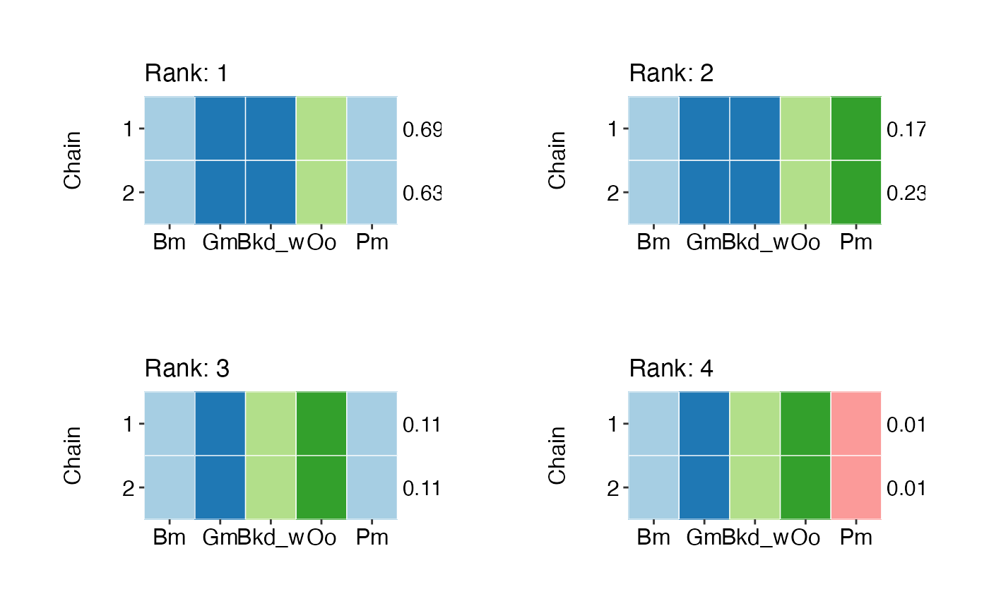
model.select = TRUE, this is done by looking at (i) running means plots of themodel_IDparameter (which should show chains plateau-ing around the same model (or set of models), (ii) tile plots of species groupings for top-ranked models (which should show comparable grouping patterns and similar posterior probabilities across chains), and (iii) to some extent, density plots of model size (i.e., number of species groupings). Similarly, whenfunction.select = TRUE, the chain-specific posterior probabilities for each dose-response functional forms should be within Monte Carlo errors of each other.Second, assess the convergence of the Metropolis-Hastings sampler (within-model jumps). Here, convergence and mixing are commonly ascertained both (1) graphically, by inspecting e.g., trace plots of individual parameters and checking that chains are clearly stable and well-mixed, and that posterior density distributions are smooth, and (2) numerically, using diagnostics such as those available in package
coda(Plummer et al. 2006).
The summary and plot methods provide all
the information needed to perform the checks described above.
Specifically, a run of summary returns:
An overview of model run parameters (e.g., number of chains, chain lengths, burn-in, priors, move probabilities, etc.)
Acceptance rates and effective sample sizes for each parameter
A numerical assessment of model convergence using the Gelman-Rubin statistic (also known as the potential scale reduction factor). Scores in the 1.00–1.1 range are generally considered to indicate good convergence.
espressogives a breakdown of the estimated scores for each parameter, as well as an overall (multivariate) score that summarises convergence across all parameters.A table of posterior inclusion probabilities (PIPs) for contextual covariates, when covariate selection is enabled (for both individual chains, and all chains combined). Convergence is achieved when posterior probabilities from different chains are similar (within the range of Monte Carlo error).
A table of posterior model probabilities and rankings, when model selection is enabled for both individual chains, and all chains combined). Convergence is achieved when posterior probabilities from different chains are similar (within the range of Monte Carlo error).
Tile plots of species groupings for top ranking models for both individual chains, and all chains combined).
A running means plot of the model_ID chains.
summary(rj.posterior)##
## ======================================================
## SUMMARY
## ======================================================
##
## Total iterations: 3e+05
## Burn-in: 50,000
## Thinning interval: 10
## Iterations: 50010:3e+05
## Number of chains: 2
## Sample size per chain: 25,000
## Total sample size: 50,000
##
## Run times:
## # A tibble: 2 × 2
## Chain Time
## <chr> <time>
## 1 Chain 1 09'32"
## 2 Chain 2 09'33"
##
## --------------------
## MCMC
## --------------------
## Priors:
##
## mu: Uniform (60, 215)
## phi: Uniform (1, 45)
## sigma: Uniform (1, 45)
## alpha: Uniform (110, 160)
## nu: Uniform (60, 215)
## tau: Uniform (1, 45)
## omega: Uniform (0.5, 5)
## psi: Normal (0, 1)
## exposed: Normal (0, 30)
##
## p(split): 0.5
## p(merge): 0.5
##
## NULL
##
## --------------------
## EFFECTIVE SAMPLE SIZES
## --------------------
## -- mu --
##
## # A tibble: 1 × 5
## Bm Gm Bkd_w Oo Pm
## <dbl> <dbl> <dbl> <dbl> <dbl>
## 1 1013. 1456. 1084. 1258. 524.6
##
## -- phi --
##
## # A tibble: 1 × 2
## parameter ESS
## <chr> <dbl>
## 1 phi 701.3
##
## -- sigma --
##
## # A tibble: 1 × 2
## parameter ESS
## <chr> <dbl>
## 1 sigma 1869.
##
## -- exposed --
##
## # A tibble: 2 × 2
## parameter ESS
## <chr> <dbl>
## 1 exposed_1 550.4
## 2 incl.exposed 14178.
##
## -- model --
##
## # A tibble: 3 × 2
## parameter ESS
## <chr> <dbl>
## 1 model_ID 298.1
## 2 model_size 477.2
## 3 accept.model 48281.
##
##
## --------------------
## ACCEPTANCE RATES
## --------------------
## # A tibble: 1 × 13
## `1` `2` `3` `4` `5` `6` `7` `8` `9` `10`
## <dbl> <dbl> <dbl> <dbl> <dbl> <dbl> <dbl> <dbl> <dbl> <dbl>
## 1 0.7964 0.7965 0.7965 0.7946 0.7964 0.9473 0.9720 0.1634 0.05056 0.06404
## `11` `13` `14`
## <dbl> <dbl> <dbl>
## 1 0.06356 0.01748 0.07844
##
## --------------------
## CONVERGENCE ASSESSMENT
## --------------------
## Convergence: TRUE
## Potential scale reduction factors:
##
## Point est. Upper C.I.
## mu.1 1.00 1.00
## mu.2 1.00 1.01
## mu.3 1.00 1.01
## mu.4 1.00 1.00
## mu.5 1.00 1.01
## phi 1.01 1.05
## sigma 1.01 1.02
## exposed_1 1.01 1.02
## incl.exposed 1.01 1.01
## model_ID 1.01 1.04
## model_size 1.01 1.03
## accept.model 1.00 1.00
## accept.covariates 1.01 1.01
##
## Multivariate psrf
##
## 1.01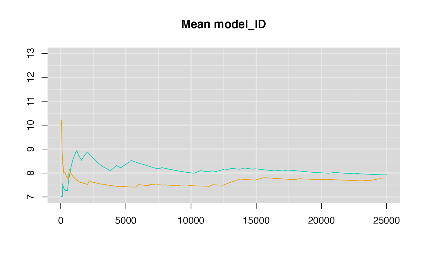
##
## --------------------
## COVARIATES
## --------------------
##
## --- All chains (n = 2) ---
## # A tibble: 1 × 5
##   covariate       p monte_carlo  lower  upper
##   <chr>       <dbl>       <dbl>  <dbl>  <dbl>
## 1 exposed   0.03144    0.001466 0.0285 0.0343
##
## --- Individual chains ---
## Chain  1 :
## # A tibble: 1 × 5
##   covariate       p monte_carlo  lower  upper
##   <chr>       <dbl>       <dbl>  <dbl>  <dbl>
## 1 exposed   0.02792    0.002101 0.0238 0.0321
##
## Chain  2 :
## # A tibble: 1 × 5
##   covariate       p monte_carlo  lower  upper
##   <chr>       <dbl>       <dbl>  <dbl>  <dbl>
## 1 exposed   0.03496    0.001814 0.0314 0.0386
##
##
## --------------------
## MODEL RANKINGS
## --------------------
##
## --- All chains (n = 2) -----------------------
##
## Top 10 models:
## # A tibble: 4 × 6
##      ID      p model                       monte_carlo  lower  upper
##   <dbl>  <dbl> <chr>                             <dbl>  <dbl>  <dbl>
## 1     7 0.6608 (Bm,Pm)+(Gm,Bkd_w)+(Oo)        0.02134  0.6186 0.703
## 2    10 0.2049 (Gm,Bkd_w)+(Bm)+(Oo)+(Pm)      0.02484  0.1557 0.2541
## 3     8 0.1162 (Bm,Pm)+(Gm)+(Bkd_w)+(Oo)      0.007037 0.1023 0.1301
## 4    13 0.0181 (Bm)+(Gm)+(Bkd_w)+(Oo)+(Pm)    0.002423 0.0133 0.0229
##
## Models common to all chains:
## # A tibble: 4 × 3
##      ID model                       rank
##   <dbl> <chr>                       <chr>
## 1     7 (Bm,Pm)+(Gm,Bkd_w)+(Oo)     1, 1
## 2    10 (Gm,Bkd_w)+(Bm)+(Oo)+(Pm)   2, 2
## 3     8 (Bm,Pm)+(Gm)+(Bkd_w)+(Oo)   3, 3
## 4    13 (Bm)+(Gm)+(Bkd_w)+(Oo)+(Pm) 4, 4
##
## Models shared by at least 2 chains:
## # A tibble: 4 × 3
##      ID model                       rank
##   <dbl> <chr>                       <chr>
## 1     7 (Bm,Pm)+(Gm,Bkd_w)+(Oo)     1, 1
## 2    10 (Gm,Bkd_w)+(Bm)+(Oo)+(Pm)   2, 2
## 3     8 (Bm,Pm)+(Gm)+(Bkd_w)+(Oo)   3, 3
## 4    13 (Bm)+(Gm)+(Bkd_w)+(Oo)+(Pm) 4, 4
##
## --- Individual chains -----------------------
##
## Top 4 models (chain 1):
## # A tibble: 4 × 6
##      ID      p model                       monte_carlo  lower  upper
##   <dbl>  <dbl> <chr>                             <dbl>  <dbl>  <dbl>
## 1     7 0.6902 (Bm,Pm)+(Gm,Bkd_w)+(Oo)        0.02629  0.6381 0.7423
## 2    10 0.1768 (Gm,Bkd_w)+(Bm)+(Oo)+(Pm)      0.02924  0.1189 0.2346
## 3     8 0.1160 (Bm,Pm)+(Gm)+(Bkd_w)+(Oo)      0.01017  0.0959 0.1362
## 4    13 0.017  (Bm)+(Gm)+(Bkd_w)+(Oo)+(Pm)    0.003389 0.0103 0.0237
##
##
## Top 4 models (chain 2):
## # A tibble: 4 × 6
##      ID      p model                       monte_carlo  lower  upper
##   <dbl>  <dbl> <chr>                             <dbl>  <dbl>  <dbl>
## 1     7 0.6314 (Bm,Pm)+(Gm,Bkd_w)+(Oo)        0.02973  0.5725 0.6903
## 2    10 0.2330 (Gm,Bkd_w)+(Bm)+(Oo)+(Pm)      0.03550  0.1628 0.3033
## 3     8 0.1164 (Bm,Pm)+(Gm)+(Bkd_w)+(Oo)      0.009604 0.0973 0.1354
## 4    13 0.0192 (Bm)+(Gm)+(Bkd_w)+(Oo)+(Pm)    0.003488 0.0123 0.0261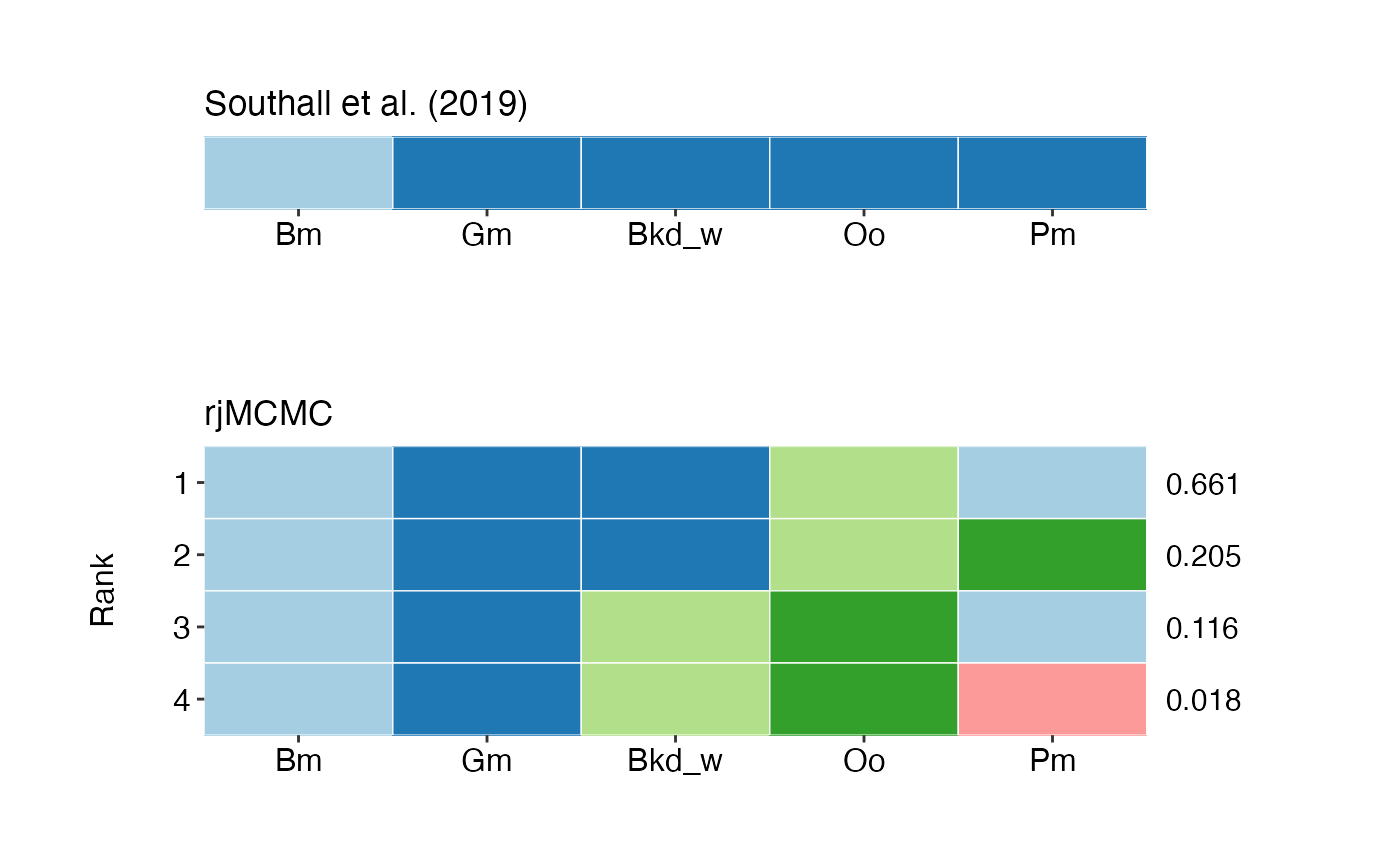
Note: The summary method presents all
outputs for individual chains and all chains combined in the same run. A
more compact version of the output summary can be obtained by hiding
sections that are not of interest. This is done by setting the relevant
argument to FALSE (see help files at
?summary.rjtrace for details). For example,
accept.rate = FALSE will hide summary of acceptance rates.
n.top sets the number of top-ranking models to display in
the output. Values (substantially) greater than 10 (the default) may
result in memory errors or long run times.
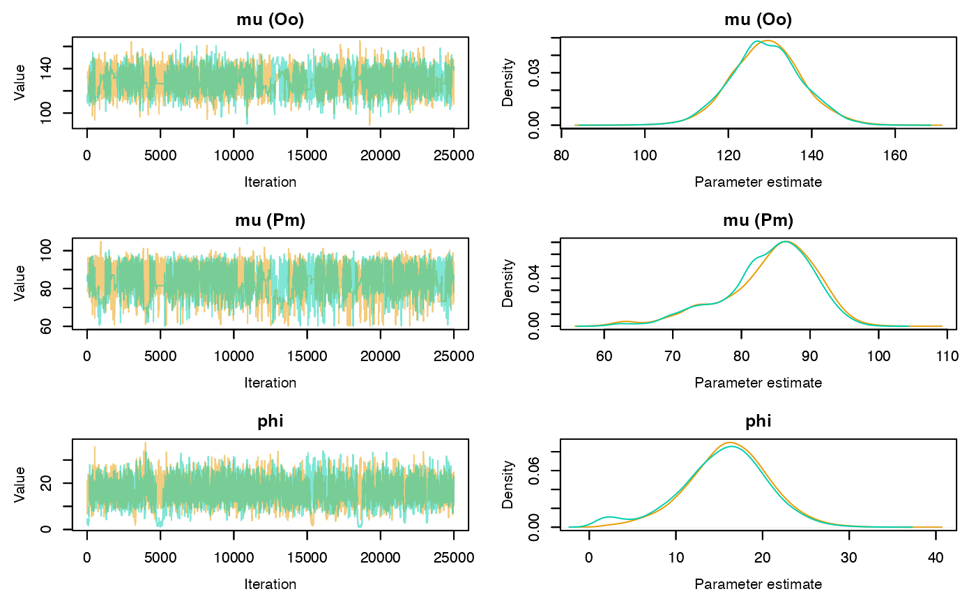
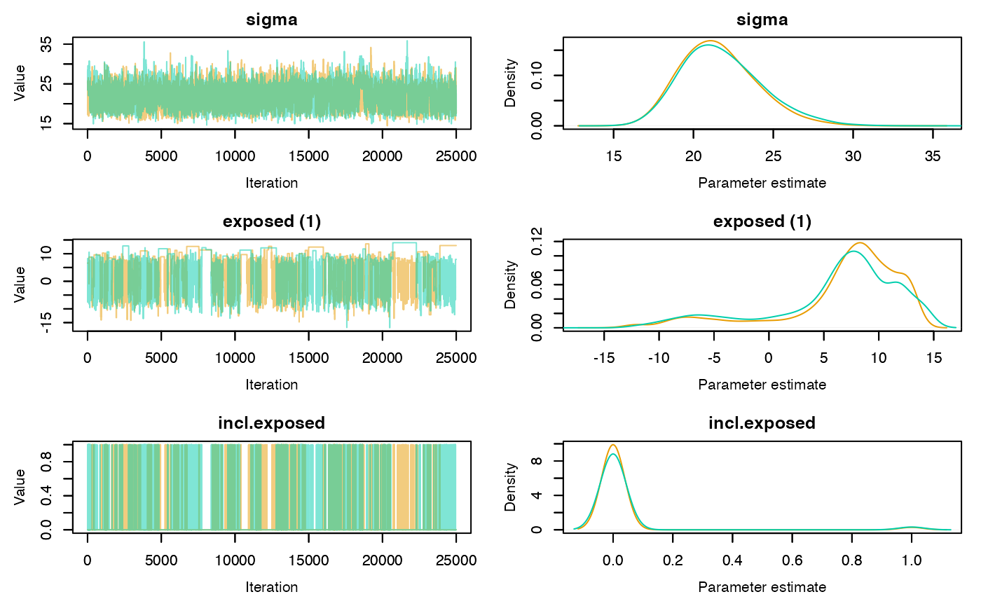
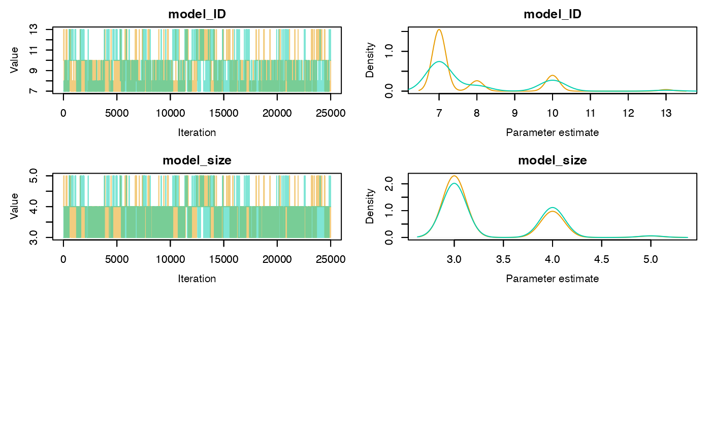
Trace and density plots can be obtained using the plot
method. Convergence is evidenced by chains that level off to a stable,
stationary state. Good mixing is apparent in plots that show random
scatter around a mean value, somewhat resembling a hairy caterpillar.
Running mean plots are also useful in identifying whether the means of
the different chains converge to a similar value. Plots for specific
parameters of interest can be generated using the
param.name argument. If individual = TRUE
separate density lines will be plotted for each chain.
plot(rj.posterior, individual = TRUE, phase = 1)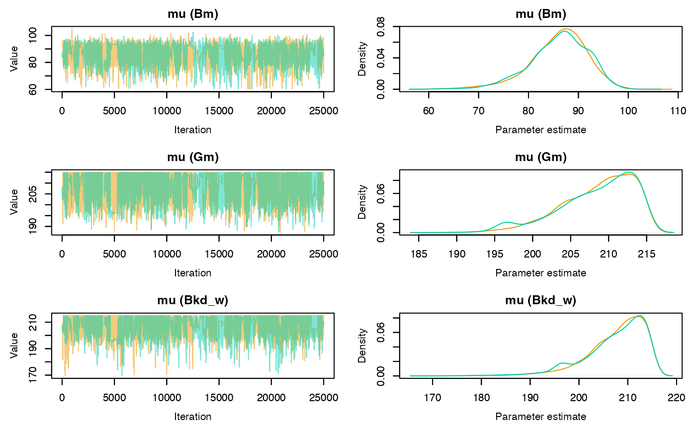
Another way to check for convergence is to look at the serial autocorrelation between MCMC samples. The lag-\(k\) autocorrelation is the correlation between every sample and the sample \(k\) steps before it. This autocorrelation should become smaller as \(k\) increases, i.e., samples can be considered as independent. If, on the other hand, autocorrelation remains high for higher values of \(k\), this indicates a high degree of correlation between our samples and slow mixing.
Note: Autocorrelation plots can be obtained with
autocorr = TRUE(the default).
# Plot for the range covariate only
plot(rj.posterior, param.name = "exposed", autocorr = FALSE)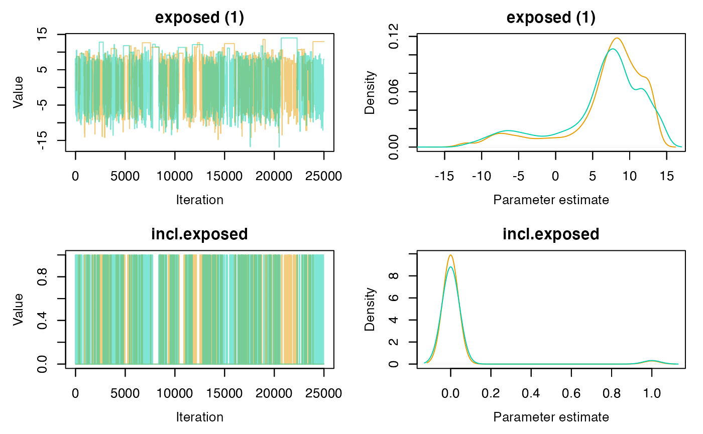
Model updates
Updates to the Markov chain may be required if the model has failed
to converge. The update_rjMCMC() function can be used to
extend a previous model run; it “picks up where the sampler left off” by
extracting the last MCMC samples for each parameter and using those as
new starting values. The same model checking procedures apply to this
new run, and the update process can be repeated until convergence is
achieved.
# Extend the previous run by 10,000 iterations.
rj.posterior2 <- update_rjMCMC(rjdat = rj, n.iter = 10000)
Dose-response
By species
The compile_rjMCMC() function computes posterior
dose-response curves for each species (or a priori species
grouping) from the parameter estimates of a fitted rjMCMC model. The
output is an object of class <dose_response>, which
can be passed to plot directly:
doseR <- compile_rjMCMC(rj.posterior, phase = 1)
class(doseR)
plot(doseR)
Note: By default,
compile_rjMCMC()calculates 5%, 50%, and 95% posterior credible intervals. These default values can be overridden using thecredible.intervalsargument. Whenfunction.select = TRUE, thephaseargument can be used to specify whether to get curves from parameter estimates associated with the monophasic (phase = 1) or biphasic (phase = 2) dose-response model.
Curves for covariates of interest can also be obtained by conditioning on a given species/species group. For example:
doseR.ex <- compile_rjMCMC(rj.posterior, covariate = "exposed", species = "Oo")
plot(doseR.ex)
For continuous covariates, such as whale-source range, curves can be generated for any
doseR.rge <- compile_rjMCMC(rj.posterior,
                            covariate = "range",
                            covariate.values = c(5, 10),
                            species = "Oo")
plot(doseR.rge, scientific.name = TRUE)
Numerous additional options are available to refine plot aesthetics,
including shading/colours, plot ordering, faceting layouts, and species
labels. Some example visualisations are given below. See
?plot.dose_response for full details.
Example 1: Black and white colour scheme.
plot(doseR, colour = "gray20", colour.median = "black")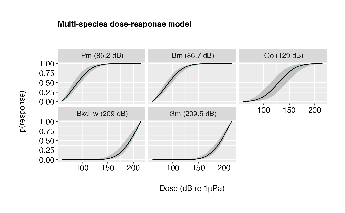
Example 2: Curves coloured by species/species groups and ordered from most to least sensitive.
plot(doseR, colour.by = "species", order.by = "response")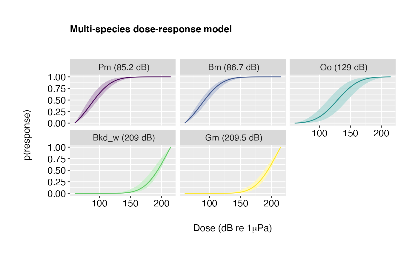
Example 3: Scientific names in plot labels, posterior medians hidden, outer credible intervals outlined.
plot(doseR, scientific.name = TRUE, show.pmed = FALSE, outline.outer = TRUE)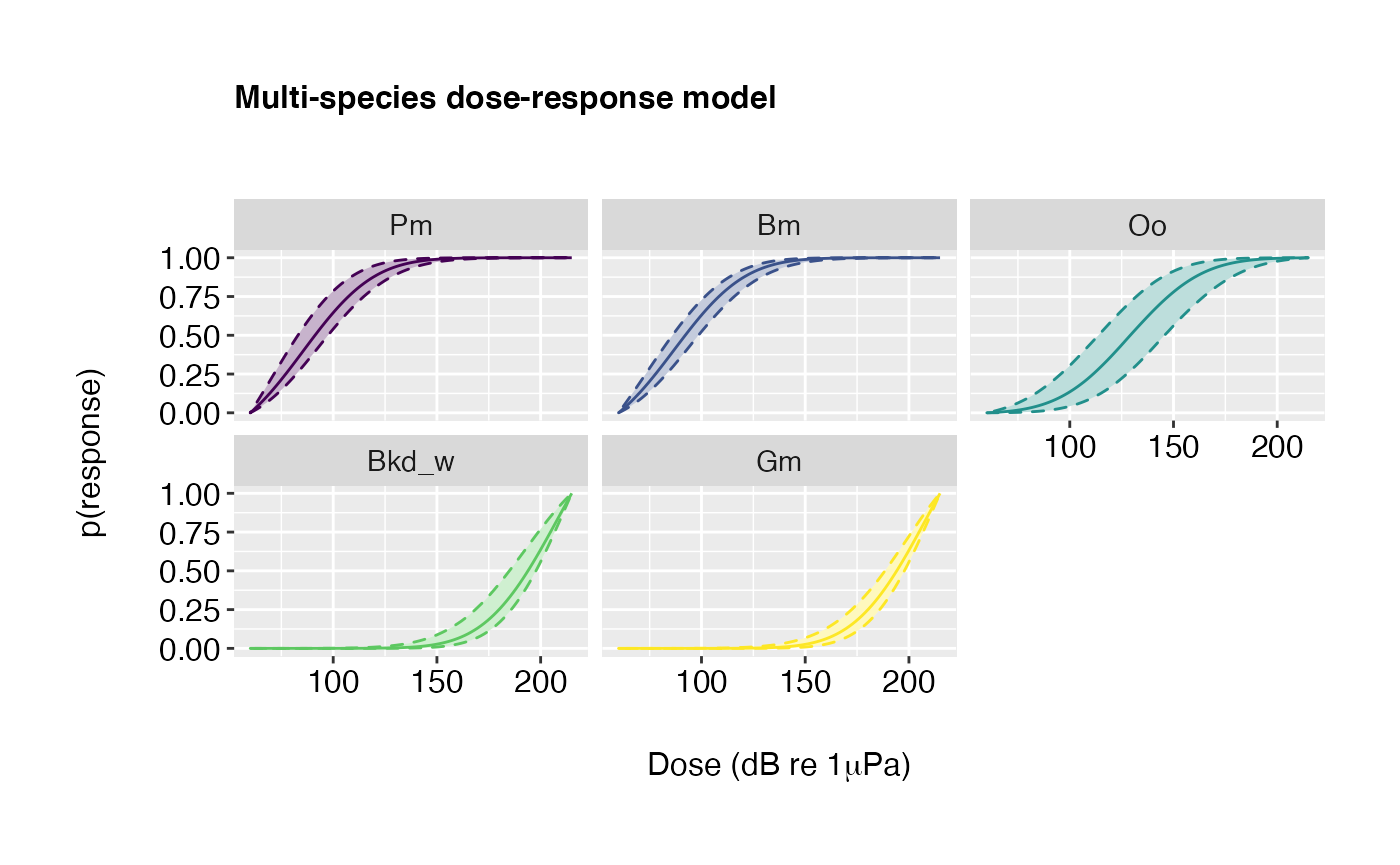
Example 4: Plot overlay.
plot(doseR, colour.by = "species", overlay = TRUE)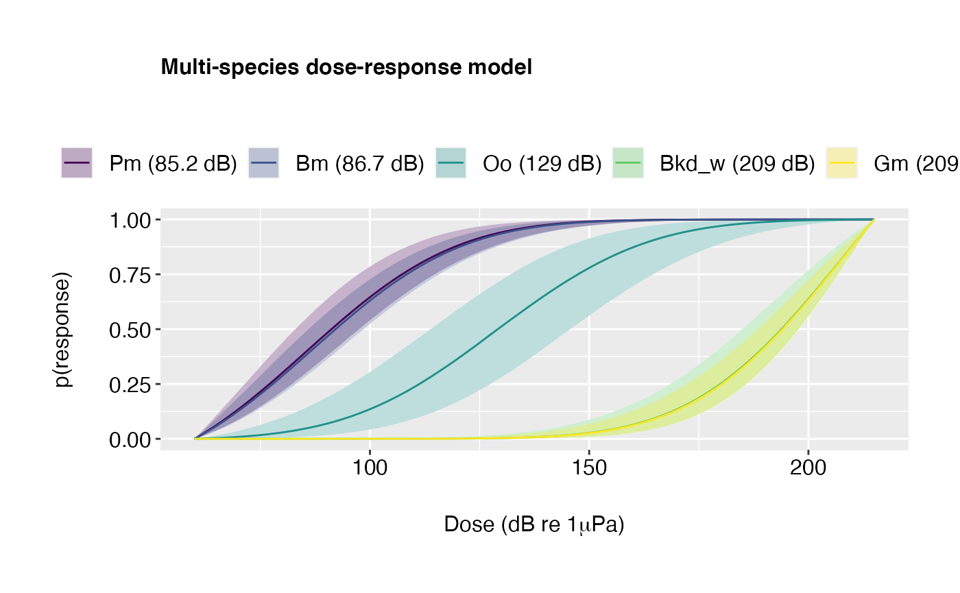
Individual plots for each species can be created using
do.facet = FALSE. All outputs can be saved to disk by
specifying do.save = TRUE and indicating the desired file
format such as file.format = "pdf" (or “png”, “tiff”,
“jpeg”). Additional arguments to ggplot2::ggsave can be
passed directly to plot to change plot dimensions, resolution, output
directory etc.
By model
When model.select = TRUE, dose-response curves are
derived irrespective of model IDs (by default), and therefore reflect
model uncertainty (see above). If dose-response functions are needed for
a specific model of interest (e.g., the top-ranking model), then the
by.model argument should be set to TRUE. This
ensures that posterior estimates are extracted for each model
separately.
doseR.bymodel <- compile_rjMCMC(rj.posterior, by.model = TRUE)Calls to plot then require an additional argument
specifying the rank of the model to be plotted. By default, this is the
model with highest posterior probability:
plot(doseR.bymodel, model.rank = 1, order.by = "response")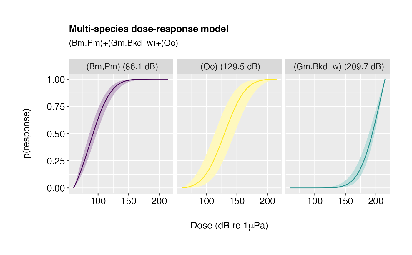
A reminder of model rankings can be obtained simply by printing the
<dose_response>object to the console.
doseR## # A tibble: 4 × 2
## model rank
## <chr> <int>
## 1 (Bm,Pm)+(Gm,Bkd_w)+(Oo) 1
## 2 (Gm,Bkd_w)+(Bm)+(Oo)+(Pm) 2
## 3 (Bm,Pm)+(Gm)+(Bkd_w)+(Oo) 3
## 4 (Bm)+(Gm)+(Bkd_w)+(Oo)+(Pm) 4